Introduction
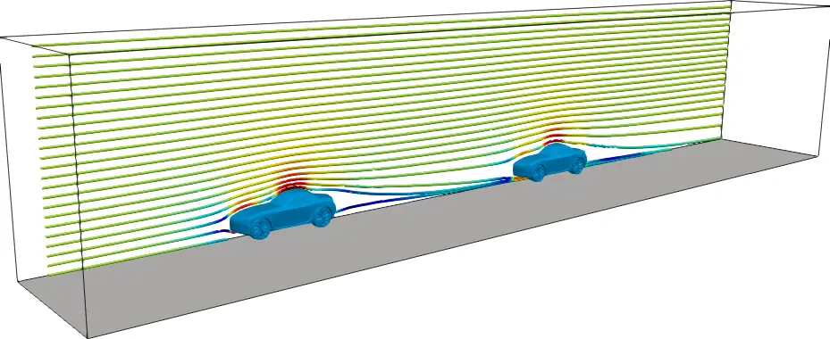
On a recent holiday, I had to drive on a dirt road while following another vehicle. I dislike driving on dirt roads but I noticed something interesting: the air flow around the front car is made apparaent by dust from the road. Its one of those times where you can visualise the flow pattern in the real world. I’ve noticed this phenomenon before on wet roads Keep an eye out when you are in these siturations. Its possible to see the turbulence as well.
The drive to our holiday was about 2.5 hours, so with a lot of time to think, I could consider how much drafting reduces fuel consumption. Obviously, I’m not going to drive dangerously close to the vehicle ahead, but how much does the drag reduce for different following distances. In cycling, cyclists slip-stream; but they are always in a tight bunch with their wheels almost touching. This is obviously not possible for cars.
Fortunately, both these questions can be answered with CFD. More specifically, I want to:
- Visualise the flow patterns around the car
- Quantify the benefits of drafting cars
CFD Setup
For the model, I will use a sports car model. Note this is not the car I took on holiday, nor one I would drive on a dirt road, but it will do. For evaluating the drag against following distance, we will just use the car model and move it down-stream of the leading car.
| Property | Value |
|---|---|
| Property | Value |
| Simulated car speed | 90 km/hr |
| Air density | 1.27 kg/m3 |
| Air viscosity | 0,6 x 0,4 m |
Due to the vehicle speed, an incompressible solver is used. I have chosen to exclude modelling the rotation of the wheels. Typically this would be included by using a multiple reference frame technique which allows a steady-state solver to still be used. Because the wheel rotation is not modelled, the cars can be thought of as sliding down the road. Maybe on a dirt road there is some truth to this...
The model is highly simplified, i.e. there are now details such as windscreen wipers, grills, bumbers etc. For a high-curiosity study, this is suitable. As the study requires more sublte optimisations, including these finer details becomes more important.
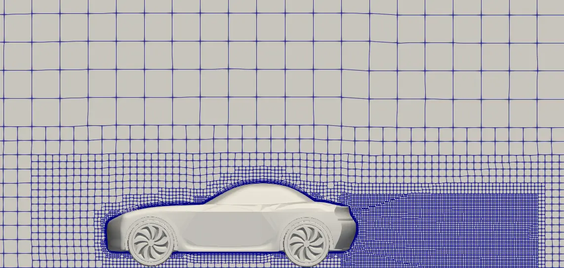
I've used a hexahedral mesh for this simulations with layers on the body of the car and a refinement region downstream of the car. The mesh is shown in the following image
Results
The first view of the car shows the velocities and the velocity streamlines. This simulation is setup in the reference frame of the car which means that the air is seen to approach it, rather than the air being still as the car travels through. This is important when considering what the velocities mean in relation to the reference frame.
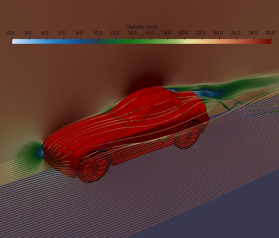
We'll start by look at the stream lines of the flow approaching the car. We see that the air is deflected up and over the top of the car and round the side. The air is incompressible, so this deflected flow needs to accelerate around the car. The energy to accelerate the flow is gained from the pressure field around the car which we will look at shortly.
The deflected streamlines separate from the car on the tail. The figure shows that there is significant rotation in the wake of the car. This rotating disturbed flow would have sufficient energy to pick up dust as the car travels allowing it to be carried on the air.
In the wake of the car, there is a region of zero velocity shown by the white and blue area directly behind the car. This means that this air is dragged along with the car. Even the green regions, because the indicate flow moving slower than the freestream are actually travelling with the car. This means that car is pulling this air along. Dust in the air at these points would actually apear to be travelling along with the car (although the car would be pulling away).
Now that we have looked at the flow patterns around the single car, we could start considering the flow where there are multiple cars.
A car drafting close enough to the front car would not have to deflect the oncoming air which would lead to some advantage. The car following in the air being dragged by the leading car would be assisted. Furthermore, the leading car would not be dragging as much air behind itself. The leading car would then benefit in addition to the trailing car.
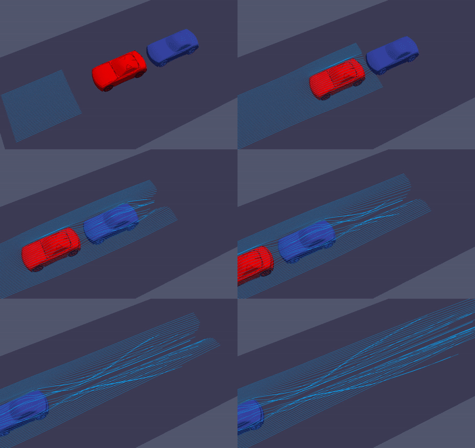
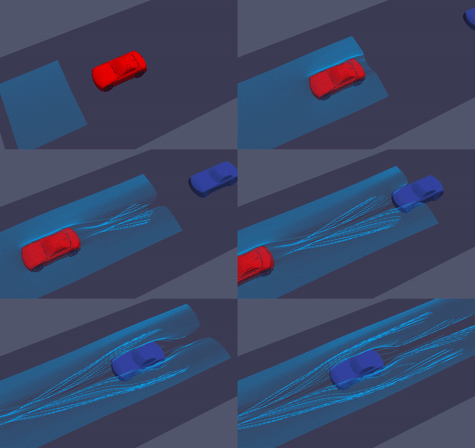
The sequence below shows how the streamlines pass over the two vehicles. Where the car are slip-streaming, the flow from the first car passes straight over the second car. This is not the case when the cars are not far apart. The affect on the overall flow stream is larger when the cars are further apart in comparison to when the second rides within the wake of the first car. Intuitively, this make sense. It also makes sense that minimising the affect on the overall flow stream would result in a reduced combined drag for both verhicles.
Drag coefficients
I've extracted the drag coefficient for each of the cases and tabulated them below.
| Number of cars | Following distance | Cd Car 1 | Cd Car 2 |
|---|---|---|---|
| 1 | N/A | 0.35 | N/A |
| 2 | 1 m | 0.21 | 0.29 |
| 2 | 10 m | 0.33 | 0.32 |
A single car on its own has a drag coefficient of about 0.35. This seems to be a fairly typical value for cars which is encouraging. Where two cars are drafting each other the drag coefficient for both vehicles drop as expected. What is interesting is that the drag coefficient of the front vehicle drops the most. This suggests that it is the drag behind the vehicle that has the largest affect on the overall drag. The drag coefficient of the second vehicle of 0.29 confirms this. This has been observed in NASCAR slip-streaming. The trailing car reduces proximity to the lead car reduces the speed of the air over the lead car's spoiler, thereby improving its efficiency.
When the trailing distance is two car lengths, the drag coefficients are very similar to that of a single car. Even this trailing distance is not recommended. At this speed, it is recommended to have a 3s - 4s gap which translates into 75 m - 100 m. A gap of 10 m is therefore still very dangerous and not recommended. This means practically (and safely) there is no way to benefit from slip-streamining in normal driving.
The flow around the second car is clearly totally different to the flow around the leading car. This is was clearly seen in the case where the trailing distance was largest. This difference in the flow pattern highlights the important of the initial flow conditions. In the case of a car travelling into stationary air, the setup above is reasonable. In other analysis such as the flow over a building, it is unlikely the oncoming wind will approach square to one of the building walls. In this case, it may be necessary to simulate multiple conditions. This can easily be done by reorientating the geomtery and remeshing.
Some thoughts...
The seed for this blog post was some observations while driving on holiday. Having performed the CFDs, its opened some more questions, but ultimately one has to stop somewhere. I have however found it to be very interesting. I have listed some other questions that have come to mind while performing this work:
- What fraction of fuel consumption is used to overcome aerodynamic drag. This becomes more and more relavent in the quest for green vehicles. However, perhaps with autonomous driving where car's control systems become sophisticated enough to slip-stream on long straights might give greater efficiency increases than better engines or battery technology.
- Frequently, trucks add parts on the front to improve the aerodynamics. It seems that drag on the back of the vehicle is more important to reduce. For trucks pulling trailers this is obviously difficult. However, with automous driving again, this might be achievable by having trucks slip-stream. Obviously, this would require sophisticated control systems but it is possible. Trains are often touted as being more efficient that road vehicles. I wonder how much this has to do with each carriage essentially being able to slip-strean the one before?
Conclusions
In this post we provided an example of analysing the flow in a simulated wind tunnel. For this case we looked at the flow over a single car and for two cars slip-streaming each other. We were able to visualise the flow pattern around the car. It was also possible to see how the flow in the wak gets dragged along behind the car. Where there were multiple cars, it was possible to evaluate the drag coefficients on each car in each position. The simulation showed that slip-streamining does reduce the overall drag, but the distances between cars needs to be very small making these manevours very dangerous.
If you have any questions, or would like to discuss how CFD could be of value to your process please contact us.
People have different reasons for running a setup such as this. There is certainly no shortage of examples from the obvious optimisations in formula one, to reducing drag on trucks, testing aerofoils, buildings, radars, chimneys etc. The list is really endless. In this case we had a curiousity which we needed to satisfy. Fortunately, this example proves how useful a CFD can be. To test this would have been a big undertaking. In a few hours with a simulation we know the answer. This is the power that simulation enables: the ability to explore ideas quickly which enables the ability to innovate.